


Updated October 2026: We tied the DTM accuracy figures to their source, Salach et al. (2018), a single levee study, and corrected them by vegetation height (about 5.5 in for photogrammetry vs. 4.3 in for LiDAR on bare ground, 14.2 in vs. 4.3 in above 24 in). We dropped an unsourced 18-inch dense-shrub figure and the claim that photogrammetry can’t meet a sub-3-inch RMSE spec, raised the checkpoint minimum to the ASPRS Edition 2 count of 30, and noted that the 0.5 m and 2 m vegetation-height cutoffs are a convention, not part of LAS 1.4. We also removed an unsourced “10–30% of pulses reach bare earth” figure for LiDAR under canopy; the share varies too widely to quote one range. Where we explain why tall vegetation degrades the photogrammetric DTM, that explanation is now marked as our inference rather than Salach’s finding.
You finish a flight, run Metashape through dense cloud generation, and export a LAZ file with 80 million points. Every rooftop, every tree crown, every gravel access road, and every piece of equipment parked on the pad is mixed together in a single undifferentiated mass of XYZ coordinates. You need a bare-earth DTM for cut/fill volumes, but vegetation is in the way.
Point cloud classification photogrammetry is the process of assigning semantic labels — ground, vegetation, buildings — to individual points in a drone-derived dense cloud. Once classified, you can filter to ground-only points and interpolate an accurate DTM. Skip this step and your “terrain model” is actually a surface model of whatever happens to be sitting on the ground.
This article covers how classification works, why photogrammetry behaves differently from LiDAR, what each major tool actually does under the hood, and when photogrammetry classification is good enough versus when you need to rent a LiDAR sensor.
ASPRS Class Codes: The Standard Labels
Every LAS and LAZ file stores a class code integer on each point. The American Society for Photogrammetry and Remote Sensing (ASPRS) defines the standard codebook in the LAS 1.4 specification. These codes are universal across tools — a class-2 point from Metashape means the same thing as a class-2 point in ArcGIS Pro or PDAL.
The codes you will work with on most projects:
| Code | Class Name | Practical Meaning |
|---|---|---|
| 0 | Created, Never Classified | Raw, unprocessed |
| 1 | Unclassified | Processed, no class assigned yet |
| 2 | Ground | Bare earth — used for DTM interpolation |
| 3 | Low Vegetation | Commonly under ~20 in (0.5 m) — grass, crops |
| 4 | Medium Vegetation | Commonly ~20 in–6.6 ft (0.5–2 m) — shrubs |
| 5 | High Vegetation | Commonly over 6.6 ft (2 m) — trees |
| 6 | Building | Roof surfaces, structures |
| 7 | Low Point / Noise | Below-ground outliers, sensor error |
| 9 | Water | Lake and river surfaces |
| 17 | Bridge Deck | Bridge surfaces, separated from ground |
| 18 | High Noise | Airborne returns, birds |
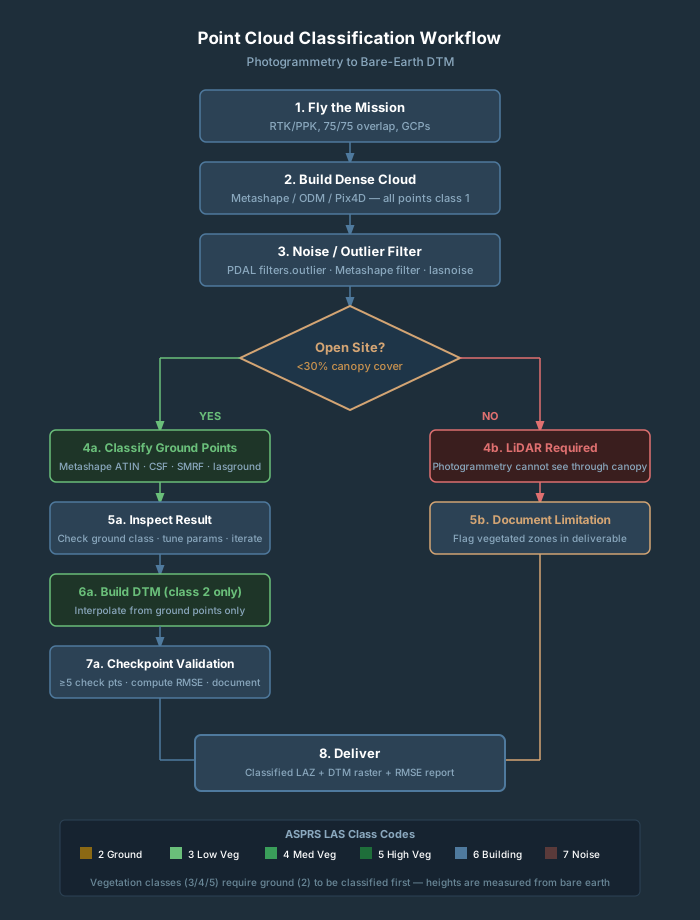
The LAS 1.4 specification names classes 3, 4 and 5 but does not define their height ranges. The 0.5 m and 2 m cutoffs in the table are a common convention, not part of the spec; your client’s specification or your own project settings decide the actual breaks. Whatever cutoffs you use, vegetation height is measured from the classified ground surface — which is why you must classify ground first before vegetation classification is meaningful. When a fresh Metashape dense cloud exports, every point is typically class 1 (Unclassified). Some Pix4D exports are class 0. Either way, you are running classification yourself in post.
How Photogrammetry Differs from LiDAR for Classification
Understanding this single difference will save you from delivering unusable DTMs.
Canopy Penetration: The Hard Limit
LiDAR fires active laser pulses. A single pulse can produce multiple returns: first return off the canopy, intermediate returns through gaps in foliage, and a last return from the ground. In forested terrain with canopy gaps, enough pulses usually reach bare earth to interpolate a DTM. The share varies widely with canopy density, season and scan angle, so there is no single typical percentage.
Photogrammetry works from reflected light and image matching. Structure from Motion (SfM) and multi-view stereo reconstruction create points only where cameras can see a surface. Under any vegetation — even tall grass — photogrammetry cannot reconstruct what is hidden from the camera lens. The ground beneath a tree canopy is simply absent from a photogrammetry point cloud. The nearest points are the crown surface.
Any DTM generated from photogrammetry in vegetated terrain is not a terrain model. It is a surface model of whatever is on top.
Density and Edge Noise
Photogrammetry at typical drone survey overlap (75/75 or 80/75) produces 100–1,000+ points per square foot — denser than most drone LiDAR systems. That density advantage disappears under canopy because all those points are at the canopy surface.
Photogrammetry clouds also carry more noise along object edges — where image matching is geometrically ambiguous — and in low-texture areas like water, asphalt, and uniform painted rooftops. LiDAR transitions more cleanly at building edges. For photogrammetry clouds, a noise-filtering pass before ground classification is not optional on production work.
DTM Accuracy by Vegetation Height
The cleanest direct comparison we know of is Salach et al. (2018), ISPRS International Journal of Geo-Information 7(9):342. The team flew a UAV LiDAR scanner and a camera (2 cm GSD) on the same drone over a river levee, built 25 cm DTMs from each, and checked them against 193 GNSS-RTK checkpoints grouped by vegetation height:
- Bare ground and vegetation under 8 in (0–20 cm): Photogrammetry RMSE 5.5 in (0.139 m). LiDAR 4.3 in (0.109 m). The gap is small.
- Vegetation 8–16 in (20–40 cm): Photogrammetry 9.5 in (0.242 m). LiDAR 5.5 in (0.139 m).
- Vegetation 16–24 in (40–60 cm): Photogrammetry 10.7 in (0.271 m). LiDAR 4.3 in (0.109 m).
- Vegetation over 24 in (60 cm): Photogrammetry 14.2 in (0.361 m). LiDAR 4.3 in (0.110 m). More than a 3x gap. Not reliable for survey-grade deliverables.
- Tree canopy: No usable ground points from photogrammetry. Do not attempt.
Treat these as one study’s numbers, not a rule. Salach’s images were processed in PhotoScan 1.2.6 from two corridor strips at 70/50 overlap, and the authors summarize the trend as roughly 0.10 m (4 in) of lost photogrammetric accuracy for every 20 cm of vegetation height, a dependency they did not see in the LiDAR. On bare, flat ground, well-controlled photogrammetry can do better than 5.5 in: a review by Jiménez-Jiménez et al. (2021), ISPRS IJGI 10(5):285, reports vertical RMSE of 1–4.5 times the GSD on flat terrain (about 0.8–3.5 in at a 2 cm GSD) and 1.5–5 times the GSD on complex topography. Vegetation erodes those figures the way Salach shows. On a mixed site, Klápště et al. (2020) measured ground-filtering RMSE of 0.19–0.23 m (7.5–9.1 in) for leaf-off drone photogrammetry vs. 0.13–0.19 m (5.1–7.5 in) for leaf-on airborne LiDAR of the same area.
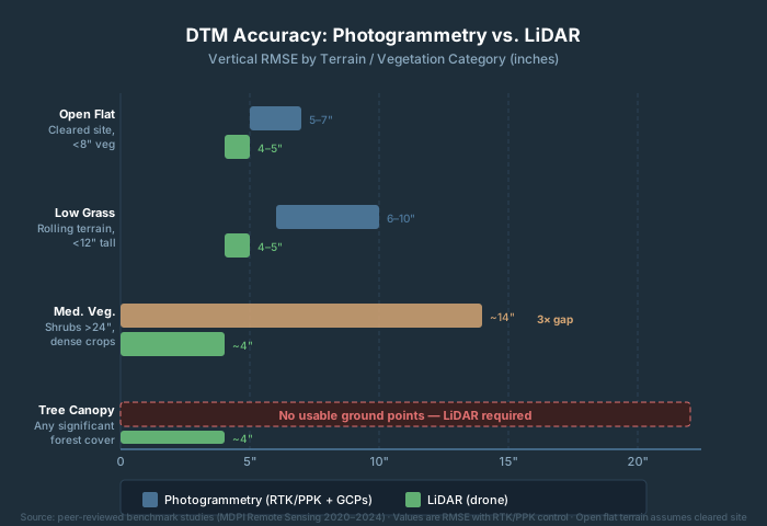
The honest rule: if you fly the site and can see dirt in the imagery, classification will work. If you see green, you need LiDAR — or you need to document the limitation explicitly in your deliverable.
Tool-by-Tool Walkthrough
Metashape — Built-In ATIN Classification
Metashape’s ground classifier uses an Adaptive Triangulated Irregular Network (ATIN) algorithm — not CSF. This matters because the parameter names only make sense in an ATIN context.
The algorithm works in two stages. First, it divides the cloud into grid cells and finds the lowest point in each cell to build a coarse seed TIN. Then it iteratively adds more points to the ground class if they satisfy two conditions: within Max Distance of the current TIN surface, and the angle between the TIN face and the candidate point is within Max Angle.
Key parameters and how to tune them:
| Parameter | Default | When to Adjust |
|---|---|---|
| Max Angle (°) | 15 | Increase to 20–30° for steep terrain |
| Max Distance (m) | 1.0 | Increase for rough, uneven terrain |
| Max Terrain Slope (°) | 45 | Lower to reduce vegetation bleeding into ground class |
| Cell Size (m) | 50 | Set to match the largest gap with no ground — e.g., a large building footprint |
| Erosion Radius (m) | 0 | Set to 1–2 m to reduce building/tree stump artifacts |
The workflow: Tools → Point Cloud → Classify Ground Points. After running, inspect in 3D view with ground points highlighted. Then Model → Build DEM, Source: Point Cloud, Classes: Ground (class 2).
Common issues on photogrammetry data: tall grass bleeding into the ground class (increase Max Terrain Slope or tighten Max Distance), and building walls classified as ground (set Erosion Radius to 2 m).
CloudCompare — CSF Plugin (Free)
CloudCompare ships with the Cloth Simulation Filter (CSF) as a bundled plugin. This is the most accessible free option for ground classification.
CSF is a physics simulation: the point cloud is flipped upside down, a virtual cloth is dropped onto the inverted surface, and gravity plus internal spring tension causes the cloth to settle against the terrain. Points within a set distance of the settled cloth are ground; everything else is non-ground.
Key parameters:
| Parameter | Default | What It Controls |
|---|---|---|
| Cloth Resolution | 0.5 m | Grid spacing — smaller captures finer terrain detail |
| Classification Threshold | 0.5 m | Distance cutoff: points within this distance = ground |
| Rigidness | 2 (Medium) | Cloth stiffness: 1=rugged terrain, 2=default, 3=flat only |
| Slope Processing | On | Leave enabled for photogrammetry |
| Post-processing | On | Fills density gaps in cloth |
Workflow: load your LAZ, select the cloud, Plugins → CSF Filter, set parameters, run. For survey delivery with standard ASPRS codes, you will need to reclassify or push the result through LAStools or PDAL to write class-2 codes. For visual QA or one-off work, CloudCompare CSF is fine as-is.
LAStools — Production Pipeline
LAStools (rapidlasso GmbH) is the industry-standard toolkit for production classification. The standard three-step workflow:
Step 1 — lasground classifies ground vs. non-ground using the Axelsson progressive TIN densification algorithm. For photogrammetric clouds, tune the -bulge parameter. Use -nature preset for natural terrain, -town for urban areas:
lasground -i survey.laz -o survey_ground.laz -nature
Step 2 — lasheight computes height above ground for every non-ground point. Required before vegetation heights can be determined:
lasheight -i survey_ground.laz -o survey_height.laz
Step 3 — lasclassify assigns buildings (class 6) and high vegetation (class 5) among elevated non-ground points. Minimum reliable density for building detection: ~2 points/m² — photogrammetry routinely delivers 100–1,000+:
lasclassify -i survey_height.laz -o survey_classified.laz
Licensing. LAStools is not open source. lasground, lasclassify, and lasheight require a commercial license for paid or government work. Without a license, outputs are degraded. Verify current pricing at rapidlasso.de before building a deliverable workflow around it.
ArcGIS Pro — Classify LAS Ground
ArcGIS Pro’s Classify LAS Ground tool (3D Analyst extension) offers four detection methods: Standard, Conservative, Aggressive, and Recover Ridges. Standard is the right starting point for most photogrammetry inputs. After running Standard, use Recover Ridges to pick up ridge lines the initial pass missed.
Classify LAS By Height provides vegetation height classification (classes 3/4/5) after ground is established, analogous to the lasheight + lasclassify pipeline in LAStools.
ArcGIS Pro also supports deep learning-based classification via Classify a Point Cloud with Deep Learning. For complex urban scenes, deep learning outperforms rule-based methods. Requires 3D Analyst extension — confirm your client’s licensing before specifying this workflow.
See also: AI Point Cloud Processing for a full breakdown of deep learning classification options.
PDAL — Open-Source Scripted Pipelines
PDAL (Point Data Abstraction Library) is a BSD-licensed command-line and Python library for point cloud processing. For ground classification, the recommended filter is filters.smrf. A complete pipeline:
{
  "pipeline": [
    "input.laz",
    {
      "type": "filters.outlier",
      "method": "statistical",
      "mean_k": 12,
      "multiplier": 2.2
    },
    {
      "type": "filters.smrf",
      "ignore": "Classification[7:7]",
      "slope": 0.2,
      "window": 16,
      "threshold": 0.45,
      "scalar": 1.2
    },
    {
      "type": "filters.range",
      "limits": "Classification[2:2]"
    },
    "ground_only.laz"
  ]
}
Run it with:
pdal pipeline classify_ground.json
PDAL is free, cross-platform, and integrates cleanly with Python and ODM/WebODM post-processing scripts. Steeper learning curve than Metashape or CloudCompare, but the right tool for automated batch work.
Decision Framework: Which Tool to Use
Use Metashape’s built-in classifier if:
- Your project is already running through Metashape
- The site is open or lightly vegetated (less than 30% canopy cover)
- You need ground-only classification for DTM generation
- You do not need formal building or vegetation class codes in the deliverable
Use CloudCompare + CSF if:
- You need a free option for QA or one-off classification
- You want to visually verify ground separation before committing to a pipeline
- You do not need ASPRS-coded output for delivery
Use LAStools if:
- You need complete classification: ground, vegetation, and buildings
- You are running production volume with batch automation
- Your deliverable specifies LiDAR Base Specification-compliant class codes
- You have a commercial license
Use ArcGIS Pro if:
- Your final deliverable workflow lives inside ArcGIS Pro anyway
- Your client or agency requires an Esri-based workflow
Use PDAL if:
- You are building a scripted, automated pipeline
- You need open-source only (no commercial license budget)
- You are integrating with ODM, WebODM, or Python processing scripts
When photogrammetry classification is not sufficient:
- Any significant tree canopy exists over the survey area
- Deliverable spec requires a vertical RMSE of a few inches on ground covered by grass or brush taller than about 8 in (in Salach et al., photogrammetry was already at 9.5 in RMSE in 8–16 in vegetation)
- Project involves flood modeling, stormwater design, or coastal elevation
- USGS 3DEP-compliant deliverable is required
For a detailed comparison of when to choose LiDAR over photogrammetry entirely, see LiDAR vs. Photogrammetry.
Accuracy Expectations: What to Document and Deliver
Set these expectations with clients before you fly, not after you process.
On a cleared construction site or agricultural field with less than 8 inches of vegetation, ground-controlled photogrammetry can deliver a DTM vertical RMSE of a few inches: about 5.5 inches in Salach et al.’s levee study, and 1–4.5 times the GSD on bare, flat terrain in the studies reviewed by Jiménez-Jiménez et al. Measure it at your checkpoints rather than assuming it, and compare it with the RMSE the deliverable actually requires. In grass 8–16 inches tall, Salach’s photogrammetry RMSE rose to about 9.5 inches, so visual QA of the ground mask matters.
Once vegetation exceeds 24 inches in height, RMSE climbed to about 14 inches in that study. Our reading, not a finding Salach reports: in vegetation that tall the cameras mostly see the canopy, so the DTM rests on sparse ground points and interpolation across the gaps. Document it explicitly rather than delivering a DTM that looks authoritative but is not.
For checkpoint validation, ASPRS Positional Accuracy Standards, Edition 2 (Version 2, 2024) call for at least 30 independent checkpoints (not GCPs used in processing), capped at 120 for very large areas, spread across the site, including areas near vegetation and structure edges. If you test with fewer, the accuracy statement must say the test used “ONLY __ checkpoints.” Record: total points classified as ground, what percentage of the cloud that represents, RMSE at checkpoints, and known areas of limitation.
Frequently Asked Questions
What ASPRS class code is ground in a LAS file?
Class 2. This is universal across all tools and the ASPRS LAS 1.4 specification. When filtering for DTM generation, filter for Classification == 2. Low vegetation is class 3, medium vegetation class 4, high vegetation class 5, buildings class 6.
Does Metashape use CSF for ground classification?
No. Metashape uses an ATIN (Adaptive Triangulated Irregular Network) algorithm. CSF is available as a third-party Python script, but the native classifier is ATIN. Confusing the two leads to tuning the wrong parameters — Max Angle and Max Distance are ATIN parameters, not CSF parameters.
Can I get a usable DTM from photogrammetry under trees?
No. Photogrammetry cannot see through canopy. Every point under a tree crown is on the canopy surface, not the ground. For any project with significant tree cover, you need LiDAR. There is no workaround.
Do I need a license to use LAStools for client work?
Yes. lasground, lasheight, and lasclassify all require a commercial license for paid or government work. Without a license, outputs are degraded with injected noise and point-count caps. PDAL is a free alternative that handles the same classification tasks with no licensing restrictions.
What is the difference between a DTM and a DSM?
A DSM (Digital Surface Model) represents the top surface of everything — canopy, buildings, vehicles. A DTM (Digital Terrain Model) represents bare earth only. Classification is the step that separates the two: classify ground points (class 2), then interpolate the DTM from ground-only.
How do I classify a photogrammetry point cloud in PDAL without ArcGIS or Metashape?
Use filters.smrf in a PDAL JSON pipeline. Run a filters.outlier pass first to clean up photogrammetry edge noise, then run SMRF with slope: 0.2, window: 16, threshold: 0.45. PDAL is free, cross-platform, and handles batch processing well.
References
Research and standards cited in this article.
- ASPRS. (2024). ASPRS positional accuracy standards for digital geospatial data (Edition 2, Version 2.0). American Society for Photogrammetry and Remote Sensing. doi:10.14358/ASPRS.PAS.2024
- ASPRS. (2025). LAS specification 1.4 – R16. American Society for Photogrammetry and Remote Sensing. link
- Jiménez-Jiménez, S. I., Ojeda-Bustamante, W., Marcial-Pablo, M., & Enciso, J. (2021). Digital terrain models generated with low-cost UAV photogrammetry: Methodology and accuracy. ISPRS International Journal of Geo-Information, 10(5), 285. doi:10.3390/ijgi10050285
- Klápště, P., et al. (2020). Sensitivity analysis of parameters and contrasting performance of ground filtering algorithms with UAV photogrammetry-based and LiDAR point clouds. International Journal of Digital Earth, 13(12), 1672–1694. doi:10.1080/17538947.2020.1791267
- Salach, A., et al. (2018). Accuracy assessment of point clouds from LiDAR and dense image matching acquired using the UAV platform for DTM creation. ISPRS International Journal of Geo-Information, 7(9), 342. doi:10.3390/ijgi7090342